How to Add Elapsed Time in Excel

For literally decades I’ve been trying to figure out a way to add elapsed time in Excel, and this week, with the help of my friend Mike, we figured out how to do it. I feel like I have made fire.

The problem with Excel (and all spreadsheet applications) is that by default, they treat entered time as absolute time, not elapsed time. If I type in 10:00, Excel thinks I mean 10 am not 10 hours and 0 minutes. An example to prove it would be to ask Excel to add 10:00 + 15:00. If it’s elapsed time, you should get 25:00, but instead, you’ll get 1:00 because it’s gone around another day and it’s now 1:00 am.

I’ve just started working on a web app to add time so I don’t have to fight this problem anymore, but coincidentally a listener to the Mac Geek Gab asked the question of how to add time in Excel since it thinks it’s a date.

How Do I Stop it From Thinking It’s Absolute Time?

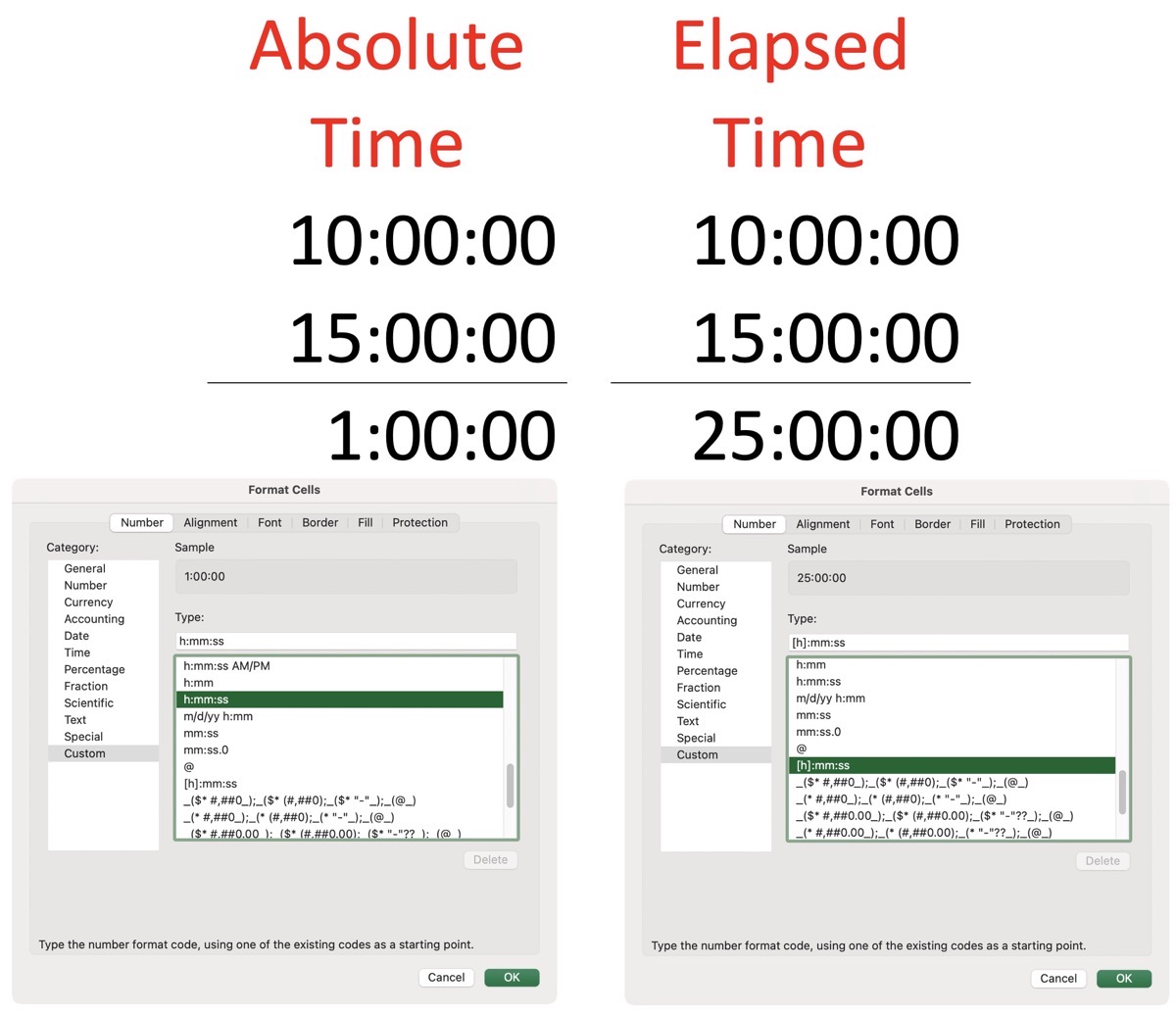
When you enter time into Excel, the default format is General. This is a magical format where Excel just does its darnedest to figure out what you mean. Under the hood it calculates a decimal value that represents the percentage of a 24 hour day.

For example, 24:00:00 would be represented as simply 1. 12:00:00 would be represented as 0.5. 48:00:00 would be represented as 2. This decimal value will become interesting to our story, and I have to give Mike 100% credit for figuring out what these decimal values mean.

In a very odd twist of logic, changing the format of the entered time from General to “[h]:mm:ss” (which you’ll find under Custom), will tell Excel that you want to treat this entered value as elapsed, not absolute time. Note the square brackets around the “h”; without those square brackets you would be explicitly telling Excel that you want it to be absolute time.

Now with this new format, you can add 10:00:00 to 15:00:00 and you’ll get 25:00:00.

Why Does the Formula Bar Show AM and PM?

Time Values Look Absolute but they’re not. This is all dandy, but you may find yourself in a confusing situation if you try to edit the cell values. Even with 15:00:00 formatted with absolute time, if you click in that cell, the formula bar will show the value as 3:00:00 PM. If you have Edit in Cell enabled, you’ll also see the absolute time of 3 PM in the cell when you double click.

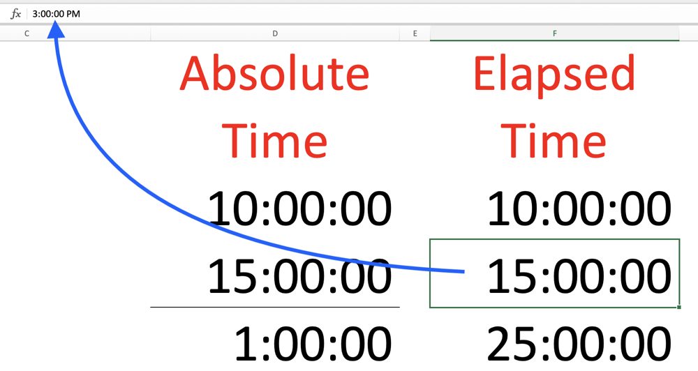
Perhaps you can live with it this way, but it’s very weird to me if I want to change 15:00:00 to 15:00:01 and the number I see is 3:00:00 PM! It works, but it’s weird.

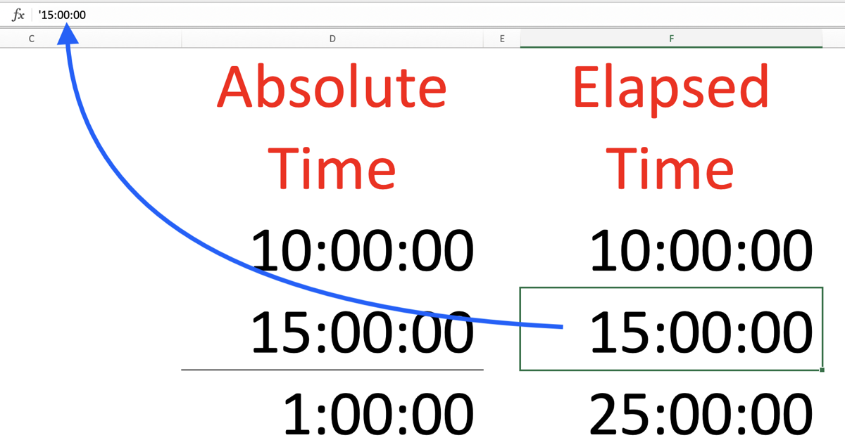
If you suspect it will lead to confusion for you like it does for me, there’s a little trick Mike and I worked out that might help. When you type in your times, put a single quote before them. In the cell, the single quote won’t show, but if you edit, you’ll see the elapsed time with the single quote before it. It’s still a little bit weird, but not as jarring as if it shows the absolute time with AM and PM!

The Hidden Danger of Subtraction

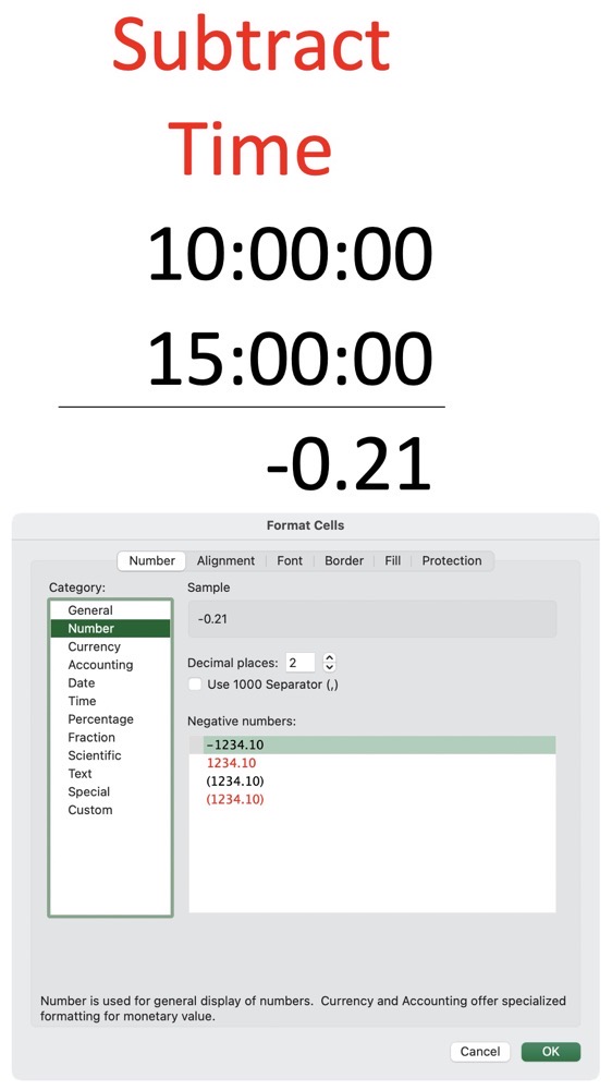
You would think the story ends right here, but what if you want to subtract elapsed times? If you subtract a smaller elapsed time from a larger elapsed time, you’ll not run into a lick of trouble. But if your calculation ends up with a negative time value, Excel will simply show you an infinitely long set of hash symbols.

You might think I don’t realize that the set of hash symbols is how spreadsheets let you know that the result of your calculation has too many digits to fit in the width of its column. That’s true, but that’s not what’s happening here. No matter how wide you stretch the column you just get more and more hash symbols.

I’m going to give you the answer of how to fix this (and it’s trivially simple) but first I’m going to make you suffer along with everything else I tried to do first.

Here’s where it gets interesting. Remember I said that all of these times are really decimal numbers under the hood? If you select this negative time value that’s just spitting out hash symbols and change the format to a decimal number, the true negative value will be revealed. As a simple example, if you enter 1:00:00 – 2:00:00, the decimal answer will be -1/24 or -0.04.

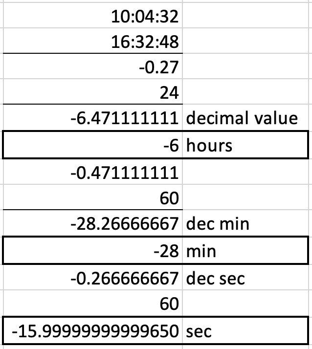
Now what good does it do you to have a time value that’s a decimal? We can build the time back up piece by piece. Let’s say we need to subtract some complex times, such as 10:04:32 – 16:32:48 and we get a decimal value of -0.27.

If we multiply that by 24 hours, we get -6.47 hours. We now know that the value starts with -6 hours. Remove the 6, and we can multiply -.47 x 60 min = -28.27. Now we know that we’re looking at -6 hours and 28 minutes. One more time, remove the 28 and take .27 x 60 seconds, and we get roughly 16 seconds. Our final answer is -6:28:16. Yay, that was easy, right?

Here’s a fun thing about those calculations. You heard me say “roughly” 16 seconds. I did the calculation in Excel, and it came out -15.999999. It took me a while to figure out why, but a quick refresher listen to Tom Merritt explaining Teraflops on his show Know a Little More. In this episode, he does a high-level explanation of how floating-point math is just an approximation.

https://play.acast.com/s/know-a-little-more/aboutteraflops-rerun-

Once I came to peace with the idea of rounding the answer, I spent about a half-day trying to figure out how to now display the answer into a cell. Remember I can’t just put it back as a negative time value, right?

I used the CONCATENATE function to put the numbers back together with colons between them. This technically did work, but for numbers less than two digits, it looked dumb, like -1:1:50. I started bothering Allister Jenks about how to format it as -1:01:50 and he gave me some fun methods including concatenating an extra zero on the front but what if it already has two digits so we’d have to only take the left two values but what about that pesky negative sign well we could take the absolute value first and then multiply by negative one but what if it was supposed to be positive….

And then I stopped. And I did a search for how to display negative time values in Excel.

The Easy Way

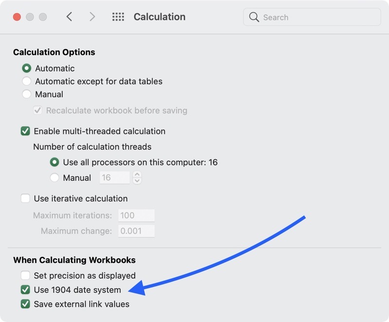
Get this. Open Excel Preferences, and in the Calculations section, set it to use the 1904 date system. Boom, the hashes are gone for time-formatted cells that are negative.

A normal person wouldn’t still be working on this but anyone who’s gone this far has to take it to the end. I can’t explain why setting the spreadsheet to the 1904 date system fixes the negative time values, but I did read up on what the heck this is even about.

I found a Microsoft support document that explains that early on, Excel for Windows used the 1900 date system, which means the earliest supported date is January 1st, 1900. But the design of the early Macintosh computer only allowed dates after January 1st 1904, which was obviously logical since the year 1900 was not a leap year. I mean, duh, right?

At some point Macs started supporting the 1900 date system, bending to the will of Microsoft I suppose. The consequence of these two different date systems is that every date has a serial number that is the elapsed number of days from the beginning of the date system.

I really wish I knew why that difference makes negative time values invalid in 1904 but not in 1900 but I’ve come to peace with it.

Can Apple Numbers Add and Subtract Elapsed Time?

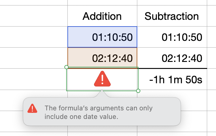
I figure at least 8% of you are wondering, how does Numbers handle time math? It’s got to be easier, right?

Formatting as elapsed time is definitely easier because Numbers has a format called Duration. That’s easier to remember and use than [h]:mm:ss, but it’s just as dumb. If you look at the formula bar, Numbers represents 13:00:00 shows as 1:00:00 AM.

Now here’s the crazy part. Numbers has zero problems calculating the subtraction of two times that results in a negative value. But guess what it can’t do? It can’t ADD two times! I’m serious. The result is a red triangle exclamation point that says “The formula’s arguments can only include one date value.” Wait, what? I can’t add two date values but I can subtract them?

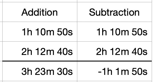
By this time I was pretty exhausted from my Excel adventures, so I did a search for how to add two time values in Numbers. It appears that Numbers isn’t really sure what you mean if you use the format 02:12:40. Heck, it could be a date, or a time, who knows? But if you write it out in a human-friendly way, then Numbers knows just what to do. Instead of 02:12:40, you write 2h 12m 40s.

This has two glorious side effects. Firstly, you can actually add and subtract time with utter abandon. The second glorious effect is that in the formula bar, it shows exactly the time you wrote, and it is not a date!

---

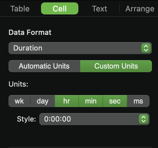
After I originally wrote this up, Mike Price, AKA Grumpy in the Podfeet Slack provided new information on how to use Numbers to add and subtract time. He discovered that if you format the cells as Duration before typing in time, you actually can enter the time as h:mm:ss and it will honor the Duration format. I hadn’t noticed it, but Mike pointed out that Duration formatting has options and you can choose the h:mm:ss version or h m s format.

While he was experimenting, he also discovered something else cool. I’ll quote him here, “I was also impressed that if some pesky data entry person (you know the type 😉). enters a silly duration value like 5:72:105 Numbers knows you ‘really’ meant 6:13:45.” Now that is nifty.

Bottom Line

I think the bottom line to the question of “how do you add time in Excel” should be, “You don’t. Use Numbers instead and write in a human-friendly format.”

I’m going to write a web app to add and subtract time, and now I have a much easier way of proving whether my math is correct in the web app. I’ll be using Numbers.